Offline Phase: GEIM algorithm

Aim of the tutorial: this notebook shows how to perform the offline phase of the GEIM algorithm, i.e. how to use this method to generate the magic functions and the associared magic sensors from a parametric dataset.

The only observable variable is assumed to be the temperature: the GEIM class is only able to handle scalar variables at the moment.

---

To execute this notebook it is necessary to have the snapshots stored in Snapshots folder, placed in this directory (otherwise modify path_FOM variable).

import numpy as np
import pickle
import os
from matplotlib import cm

from mpi4py import MPI
from dolfinx.io import gmshio
import gmsh
from dolfinx.fem import Function, FunctionSpace

from pyforce.tools.functions_list import FunctionsList
from pyforce.tools.write_read import ImportH5, StoreFunctionsList as store

Let us generate the mesh for importing OpenFOAM dataset into dolfinx

mesh_comm = MPI.COMM_WORLD
model_rank = 0

# Initialize the gmsh module
gmsh.initialize()

# Load the .geo file
gmsh.merge('cavity.geo')
gmsh.model.geo.synchronize()

# Set algorithm (adaptive = 1, Frontal-Delaunay = 6)
gmsh.option.setNumber("Mesh.Algorithm", 6)
gdim = 2

# Linear Finite Element
gmsh.model.mesh.generate(gdim)
gmsh.model.mesh.optimize("Netgen")

# Import into dolfinx
model_rank = 0
domain, ct, ft = gmshio.model_to_mesh(gmsh.model, MPI.COMM_WORLD, model_rank, gdim = gdim )
gmsh.finalize()

tdim = domain.topology.dim
fdim = tdim - 1
domain.topology.create_connectivity(fdim, tdim)

Info    : Reading 'cavity.geo'...
Info    : Done reading 'cavity.geo'
Info    : Meshing 1D...
Info    : [  0%] Meshing curve 1 (Line)
Info    : [ 30%] Meshing curve 2 (Line)
Info    : [ 60%] Meshing curve 3 (Line)
Info    : [ 80%] Meshing curve 4 (Line)
Info    : Done meshing 1D (Wall 0.00111864s, CPU 0.000849s)
Info    : Meshing 2D...
Info    : Meshing surface 1 (Transfinite)
Info    : Done meshing 2D (Wall 0.0187267s, CPU 0.007379s)
Info    : 16384 nodes 32770 elements
Info    : Optimizing mesh (Netgen)...
Info    : Done optimizing mesh (Wall 2.643e-06s, CPU 3e-06s)

Let us define the functional space onto which the OpenFOAM data have been projected; then, the snapshots can be imported.

Even if only a single variable (the temperature is analysed), var_names is defined as a list of strings, to help generalise the notebook.

path_FOM = './Snapshots/'

# The temperature is the only one that can be measured
var_names = ['norm_T']
tex_var_names = ['T']

fun_spaces = [FunctionSpace(domain, ('Lagrange', 1))]

train_snaps = dict()

for field_i, field in enumerate(var_names):

    path_snap = path_FOM+'TrainSet_'+field
    train_snaps[field] = ImportH5(fun_spaces[field_i], path_snap, field)[0]

GEIM algorithm

Generation of the magic functions/sensors

The GEIM is used to generated through a greedy process a set of basis functions and basis sensors for the data assimilation process.

Sensors are mathematically modelled as linear continuous functionals \(v_m(\cdot)\), defined as \begin{equation*} v_m(u(\mathbf{x});\,\mathbf{x}_m,\,s)=\int_\Omega u(\mathbf{x})\cdot \mathcal{K}\left(\|\mathbf{x}-\mathbf{x}_m\|_2, s\right)\,d\Omega \end{equation*} given \(\mathbf{x}_m\) the centre of mass of the functional and \(s\) its point spread. The current version adopts Gaussian kernels \begin{equation*} \mathcal{K}\left(\|\mathbf{x}-\mathbf{x}_m\|_2, s\right) = \frac{e^{\frac{-\|\mathbf{x}-\mathbf{x}_m\|_2^2}{2s^2}}}{\displaystyle\int_\Omega e^{\frac{-\|\mathbf{x}-\mathbf{x}_m\|_2^2}{2s^2}}\,d\Omega} \end{equation*} such that \(\|\mathcal{K}\left(\|\mathbf{x}-\mathbf{x}_m\|_2, s\right)\|_{L^1(\Omega)}=1\), this models the measurement process of scalar fields.

from pyforce.offline.geim import GEIM

geim_data = dict()
train_GEIMcoeff = dict()
Mmax = 20

# This parameter serves as input to select only some cells in the mesh
sam_every = 5

s = 0.01

train_abs_err = np.zeros((Mmax, len(var_names)))
train_rel_err = np.zeros((Mmax, len(var_names)))

for field_i, field in enumerate(var_names):
    geim_data[field] = GEIM(domain, fun_spaces[field_i], field_i, s=s)
    tmp = geim_data[field].offline(train_snaps[field], Mmax, sampleEvery = sam_every, verbose = True)

    train_abs_err[:, field_i] = tmp[0].flatten()
    train_rel_err[:, field_i] = tmp[1].flatten()
    train_GEIMcoeff[field] = tmp[2]

Generating sensors (sampled every 5 cells): 3277.000 / 3277.00 - 0.008 s/it
  Iteration 020 | Abs Err: 6.48e-04 | Rel Err: 9.91e-04

Let us store the magic functions, the magic sensors and the training coefficients for later use.

path_offline = './Offline_results/'

if not os.path.exists(path_offline+'/BasisSensors/'):
    os.makedirs(path_offline+'/BasisSensors/')
if not os.path.exists(path_offline+'/BasisFunctions/'):
    os.makedirs(path_offline+'/BasisFunctions/')

pickle.dump(train_GEIMcoeff, open(path_offline+'coeffs.geim', 'wb'))

for field in var_names:
    store(domain, geim_data[field].magic_fun,  'GEIM_' +field, path_offline+'/BasisFunctions/basisGEIM_' + field)
    store(domain, geim_data[field].magic_sens, 'GEIM_' +field, path_offline+'/BasisSensors/sensorsGEIM_' + field)

Post-process: plotting magic functions and sensors

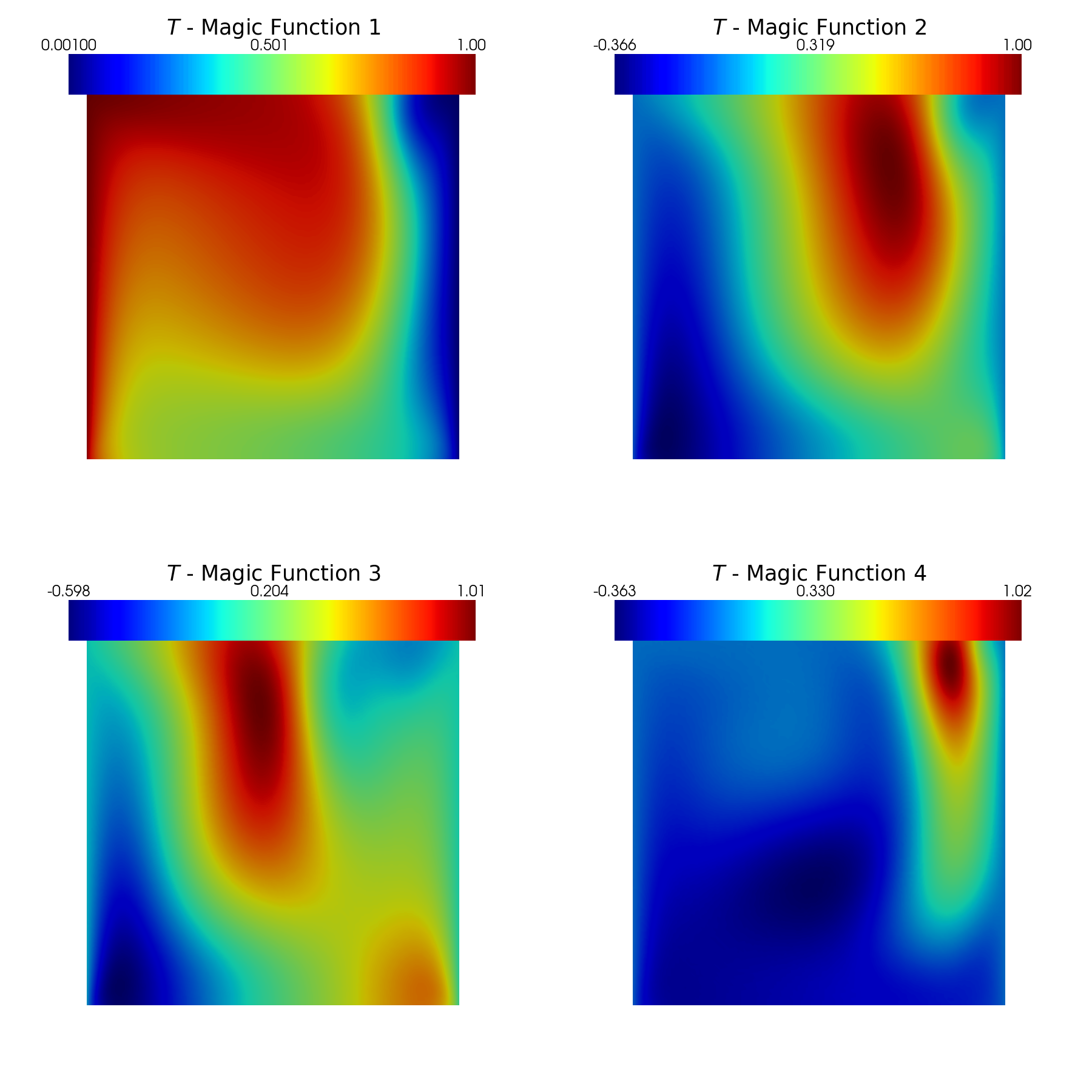
The magic functions and sensors are plotted using pyvista.

from contour_plotting import plot_modes

plot_modes(geim_data[var_names[0]].magic_fun, tex_var_names[0],
           shape=[2,2],
           title='Magic Function', zoom=1, subfig_size=[900,900],
           colormap=cm.jet)

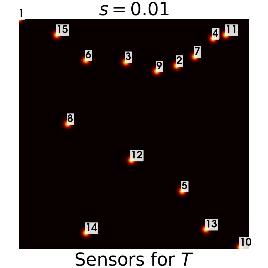
Let us also plot the sensors

from contour_plotting import plot_geim_sensors

plot_geim_sensors(geim_data['norm_T'], 15, tex_var_names[0], resolution=[900,900])