Offline Phase: generation of the POD modes

Aim of this tutorial: generate the POD modes from the snapshots of the Buoyant Cavity problem. This is a procedure which has already been performed in tutorial 1 and 2.

---

To execute this notebook: be sure to have the snapshots stored into dolfinx format.

The snapshots are related to the Buoyant Cavity problem in fluid dynamics, governed by the Navier-Stokes equations, including energy, under the Boussinesq approximation. In particular, the snapshots have been generated using the case reported in ROSE-ROM4FOAM tutorials.

import numpy as np
import pickle
import os
import matplotlib.pyplot as plt
from matplotlib import cm

from mpi4py import MPI
from dolfinx.io import gmshio
import gmsh
from dolfinx.fem import FunctionSpace
import ufl

from pyforce.offline.pod import POD
from pyforce.tools.write_read import ImportH5, StoreFunctionsList as store

Let us generate the mesh for importing OpenFOAM dataset into dolfinx

mesh_comm = MPI.COMM_WORLD
model_rank = 0

# Initialize the gmsh module
gmsh.initialize()

# Load the .geo file
gmsh.merge('cavity.geo')
gmsh.model.geo.synchronize()

# Set algorithm (adaptive = 1, Frontal-Delaunay = 6)
gmsh.option.setNumber("Mesh.Algorithm", 6)
gdim = 2

# Linear Finite Element
gmsh.model.mesh.generate(gdim)
gmsh.model.mesh.optimize("Netgen")

# Import into dolfinx
model_rank = 0
domain, ct, ft = gmshio.model_to_mesh(gmsh.model, MPI.COMM_WORLD, model_rank, gdim = gdim )
gmsh.finalize()

tdim = domain.topology.dim
fdim = tdim - 1
domain.topology.create_connectivity(fdim, tdim)

Info    : Reading 'cavity.geo'...
Info    : Done reading 'cavity.geo'
Info    : Meshing 1D...
Info    : [  0%] Meshing curve 1 (Line)
Info    : [ 30%] Meshing curve 2 (Line)
Info    : [ 60%] Meshing curve 3 (Line)
Info    : [ 80%] Meshing curve 4 (Line)
Info    : Done meshing 1D (Wall 0.00128273s, CPU 0.000814s)
Info    : Meshing 2D...
Info    : Meshing surface 1 (Transfinite)
Info    : Done meshing 2D (Wall 0.0174618s, CPU 0.00879s)
Info    : 16384 nodes 32770 elements
Info    : Optimizing mesh (Netgen)...
Info    : Done optimizing mesh (Wall 3.025e-06s, CPU 3e-06s)

Let us define the functional space onto which the OpenFOAM data have been projected: there are different definitions for scalar and vector fields.

Moreover, the variable names are defined

# Definition of the functional spaces
fun_spaces = [FunctionSpace(domain, ('Lagrange', 1)),
              FunctionSpace(domain, ('Lagrange', 1)),
              FunctionSpace(domain, ufl.VectorElement("CG", domain.ufl_cell(), 1))]

var_names = ['p', 'norm_T', 'U']
tex_var_names = ['p', 'T', r'\mathbf{u}']

The snapshots can be imported.

path = './Snapshots/'

train_snaps = dict()

for field_i, field in enumerate(var_names):

    path_snap = path+'TrainSet_'+field
    train_snaps[field] = ImportH5(fun_spaces[field_i], path_snap, field)[0]

POD algorithm

A dict will be created with the POD class of each field: the key are consistent with the var_names.

The offline POD class is used to compute the POD eigenvalues, eigenvectors and associated modes (i.e., basis functions).

The description of this class has already been covered, we highlight the fact that the eigendecomposition can be also performed using the scipy library, as shown in the following cell by turning the option use_scipy to True.

pod_data = dict()

for field in var_names:
    pod_data[field] = POD(train_snaps[field], field, verbose=True, use_scipy=True)

Computing p correlation matrix: 364.000 / 364.00 - 0.577 s/it
Computing norm_T correlation matrix: 364.000 / 364.00 - 0.451 s/it

ld: warning: duplicate -rpath '/Users/stefanoriva/miniconda3/envs/ml/lib' ignored

Computing U correlation matrix: 364.000 / 364.00 - 0.685 s/it

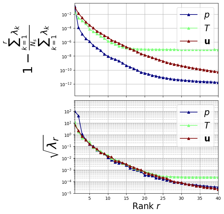
Let us plot the eigenvalues

fig, axs = plt.subplots(2, 1, figsize=(6, 8), sharex=True)

color = iter(cm.jet(np.linspace(0, 1, len(var_names))))

# Plot on the first subplot
for field_i, field in enumerate(var_names):
    c = next(color)
    axs[0].semilogy(
        np.arange(1, pod_data[field].eigenvalues.size + 1, 1),
        1 - np.cumsum(pod_data[field].eigenvalues) / sum(pod_data[field].eigenvalues),
        "-^", c=c, label="$" + tex_var_names[field_i] + "$", linewidth=1.5
    )

    axs[1].semilogy(
        np.arange(1, pod_data[field].eigenvalues[:40].size + 1, 1),
        np.sqrt(pod_data[field].eigenvalues[:40]),
        "-^", c=c, label="$" + tex_var_names[field_i] + "$", linewidth=1.5
    )

axs[0].set_ylabel(r"$1- \frac{\sum_{k=1}^{r}\lambda_k}{\sum_{k=1}^{N_s} \lambda_k}$", fontsize=30)
axs[0].set_ylim(2e-14, .4)

axs[1].set_ylabel(r"$\sqrt{\lambda_r}$", fontsize=30)
axs[1].set_ylim(1e-5, 800)

for ax in axs:
    ax.set_xticks(np.arange(0, 40 + 1, 5))
    ax.set_xlim(1, 40)
    ax.grid(which='major', linestyle='-')
    ax.grid(which='minor', linestyle='--')
    ax.legend(fontsize=20)

axs[1].set_xlabel(r"Rank $r$", fontsize=20)

fig.subplots_adjust(hspace=0.05)

Definition of the modes

\(N_{max}=20\) has been chosen by analysing the decay of the eigenvalues.

Nmax = 20

for field in var_names:
    pod_data[field].compute_basis(train_snaps[field], Nmax, normalise = True)

Let us store the POD modes.

path_offline = './Offline_results/'
if not os.path.exists(path_offline+'/BasisFunctions'):
    os.makedirs(path_offline+'/BasisFunctions')

for field in var_names:
    store(domain, pod_data[field].PODmodes, 'POD_' +field, path_offline+'/BasisFunctions/basisPOD_' + field)

Computing the training error and reduced coefficient

We need to assess the performance of the POD basis generated in the previous cells. The reduced coefficients \(\alpha_m(\boldsymbol{\mu})\) can be obtained from the train snapshots using \(L^2\) projection: given a function \(u(\mathbf{x};\boldsymbol{\mu}_n)\) with \(\boldsymbol{\mu}_n\in\Xi_{train}\), the reduced coefficients can be computed with

\begin{equation*} \alpha_m(\boldsymbol{\mu}_n) = (\psi_m, u(\mathbf{x};\boldsymbol{\mu}_n))_{L^2(\Omega)} = \int_{\Omega} \psi_m\cdot u(\mathbf{x};\boldsymbol{\mu}_n)\,d\Omega \end{equation*}

The method train_error computes the \(L^2\) error between the original snapshots and the reconstructed ones using the POD basis functions: it takes as input the train snapshots and the maximum number of modes to consider.

train_PODcoeff = dict()

train_abs_err = np.zeros((Nmax, len(var_names)))
train_rel_err = np.zeros((Nmax, len(var_names)))

for field_i, field in enumerate(var_names):
    tmp = pod_data[field].train_error(train_snaps[field], Nmax, verbose = True)

    train_abs_err[:, field_i] = tmp[0].flatten()
    train_rel_err[:, field_i] = tmp[1].flatten()

    train_PODcoeff[field] = tmp[2]

Computing train error p: 364.000 / 364.00 - 0.169 s/it
Computing train error norm_T: 364.000 / 364.00 - 0.161 s/it
Computing train error U: 364.000 / 364.00 - 0.181 s/it

Let us build the store the coefficients of the reduced basis coefficients to be later used.

for field_i in range(len(var_names)):
    pickle.dump(train_PODcoeff, open(path_offline+'coeffs.pod', 'wb'))

Post-process: plotting modes

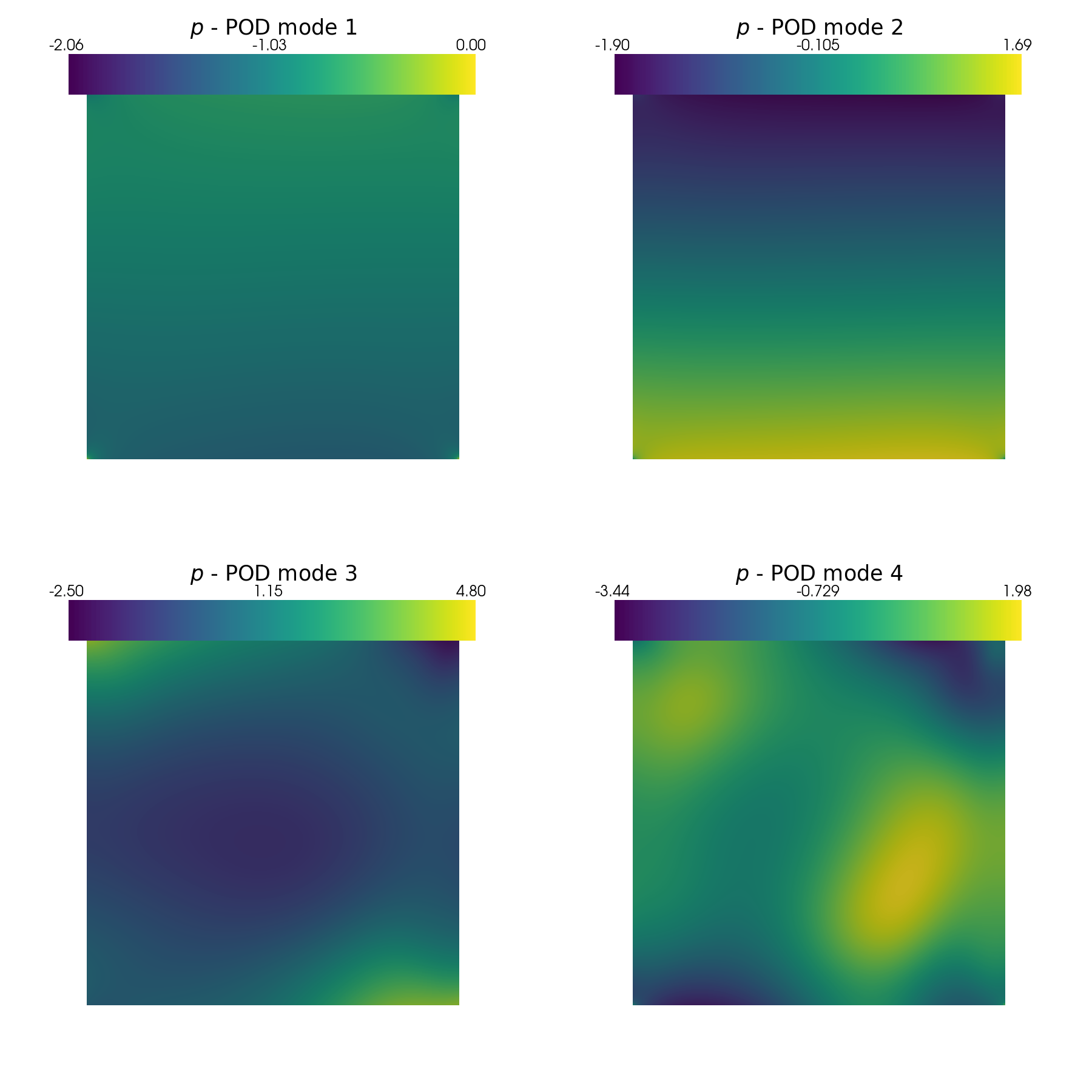
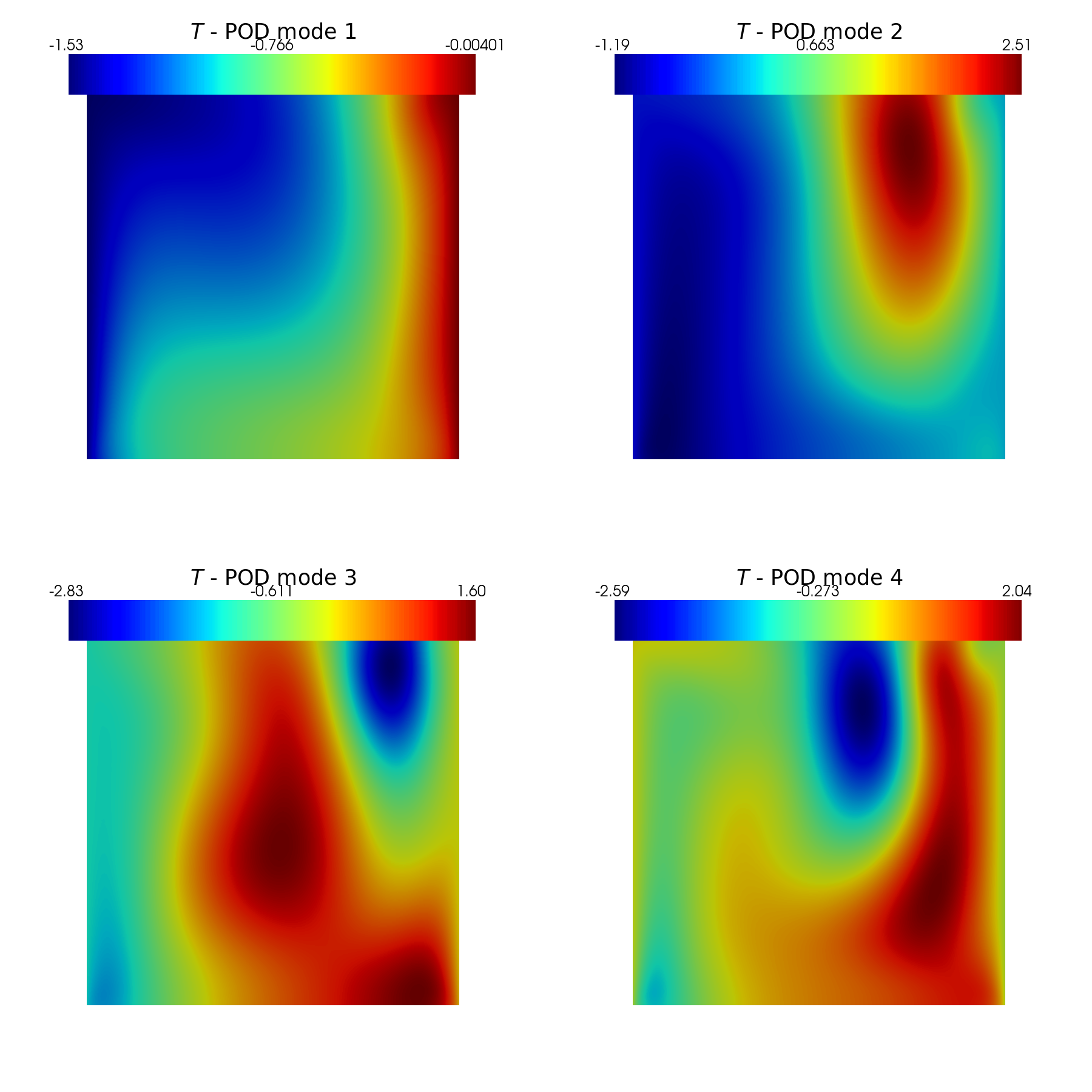
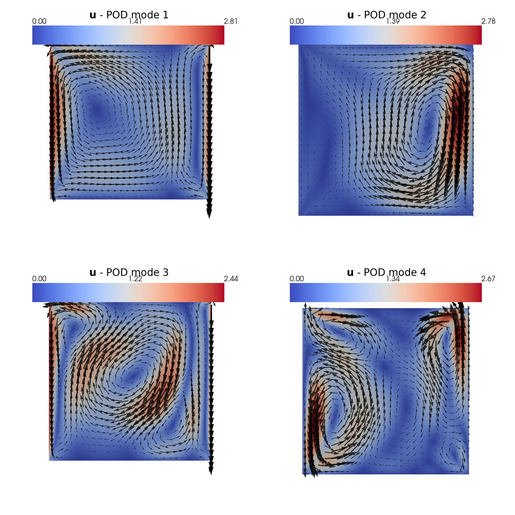
In this last section, pyvista is used to make some contour plots of the POD modes.

from contour_plotting import plot_modes

plot_modes(pod_data[var_names[0]].PODmodes, tex_var_names[0],
           shape=[2,2],
           title='POD mode', zoom=1, subfig_size=[900,900],
           colormap=cm.viridis)

plot_modes(pod_data[var_names[1]].PODmodes, tex_var_names[1],
           shape=[2,2],
           title='POD mode', zoom=1, subfig_size=[900,900],
           colormap=cm.jet)

plot_modes(pod_data[var_names[2]].PODmodes, tex_var_names[2],
           shape=[2,2], mag_plot=False,
           title='POD mode', zoom=1, subfig_size=[900,900],
           colormap=cm.coolwarm,
           factor=0.075, tolerance=0.025)