Offline Phase: PBDW offline - computing the inf-sup constant

Aim of the tutorial: this notebook shows how to calculate the \(inf-sup\) constant, bounding the approximation error of the PBDW.

---

To execute this notebook it is necessary to have the POD modes stored in Offline_results/BasisFunctions folder, placed in this directory (otherwise modify path_off variable) and the basis sensors in Offline_results/BasisSensors.

import numpy as np
from IPython.display import clear_output

from dolfinx.fem import FunctionSpace

from pyforce.tools.write_read import ImportH5, StoreFunctionsList as store

import matplotlib.pyplot as plt
from matplotlib import cm

path_off ='./Offline_results/'

The geometry is imported from “ANL11A2_octave.geo”, generated with GMSH. Then, the mesh is created with the gmsh module.

from neutronics import create_anl11a2_mesh

domain, _, _ = create_anl11a2_mesh(use_msh=True, save_mesh=False)

fuel1_marker    = 1
fuel2_marker    = 2
fuel_rod_marker = 3
refl_marker     = 4

void_marker     = 10
sym_marker      = 20

clear_output()

Importing basis function and sensors

The functional space and the names of the fields are defined.

# Defining the functional space
V = FunctionSpace(domain, ("Lagrange", 1))

# Define the variables to load
var_names = [
             'phi_1',
             'phi_2'
             ]

tex_var_names = [
                 r'\phi_1',
                 r'\phi_2'
                 ]

Let us import the POD modes using ImportH5.

bf = dict()

for field_i in range(len(var_names)):

    bf[var_names[field_i]] = ImportH5(V, path_off+'/BasisFunctions/basisPOD_'+var_names[field_i], 'POD_'+var_names[field_i])[0]

Let us import the basis sensors generated with SGREEDY.

s = 2

is_H1 = [False, True]
fun_space_label = ['L2', 'H1']

bs = dict()

for field in var_names:
    bs[field] = dict()
    for space in fun_space_label:
            bs[field][space] = ImportH5(V,
                                        path_off+'/BasisSensors/sensorsSGREEDYPOD_' + field+'_s_{:.2e}_'.format(s)+space,
                                        'SGREEDYPOD_' +field+'_s_{:.2e}'.format(s))[0]

PBDW-Offline: Compute the inf-sup constant

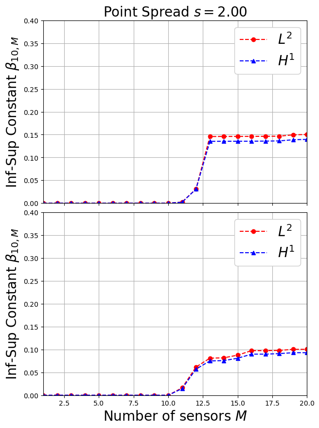
The inf-sup constant is a measure of the approximation capabilities of the PBDW, in particular highlights how the sensors are able to include more information into the background model, encoded in the basis functions. The inf-sup constant is computed by solving an eigenvalue problem, as reported in Maday and Taddei (2019).

Given the background space \(Z_N = \text{span}\{\zeta_1, \zeta_2, \dots, \zeta_N\}\), spanned by the POD modes, and the update space \(\mathcal{U}_M=\text{span}\{g_1, g_2, \dots, g_M\}\), spanned by the sensors selected by SGREEDY, the following matrices can be defined \begin{equation*} A_{mm'} = \left(g_m, g_{m'}\right)_{\mathcal{U}}\qquad K_{mn} = \left(g_m, \zeta_{n}\right)_{\mathcal{U}} = v_m(\zeta_n)\qquad B_{nn'} = \left(\zeta_n, \zeta_{n'}\right)_{\mathcal{U}} \end{equation*} The inf-sup constant \(\beta_{N,M}\) is the square-root of the minimum eigenvalue of the following problem \begin{equation*} K^TA^{-1}K \mathbf{w}_j = \lambda_j B\mathbf{w}_j \end{equation*} that is \(\beta_{N,M} = \sqrt{\min\limits_{j=1,\dots, N} \lambda_j}\).

This eigenvalue problem can be solved using the PBDW offline class, using the method compute_infsup. This class must be initialised with the basis functions, the basis sensors and the flag for the Riesz representation, either \(L^2\) or \(H^1\).

To compute the inf-sup constant the dimension of the reduced space must be fixed, a good approximation of the manifold can be reached with \(N=10\), obtained by observabing the POD eigenvalues.

from pyforce.offline.pbdw import PBDW

Nmax = 10
Mmax = 20

inf_sup_constants = dict()

for field in var_names:
    inf_sup_constants[field] = dict()

    inf_sup_constants[field]['s = {:.2f}'.format(s)] = dict()
    for kk, space in enumerate(fun_space_label):

        print('Compute Inf-Sup for '+field+' with s={:.2f}'.format(s)+' and Riesz representation in '+space)

        pbdw = PBDW(bf[field], bs[field][space], is_H1[kk])
        inf_sup_constants[field]['s = {:.2f}'.format(s)][space] = pbdw.compute_infsup(Nmax, Mmax)

        del pbdw

Compute Inf-Sup for phi_1 with s=2.00 and Riesz representation in L2
Compute Inf-Sup for phi_1 with s=2.00 and Riesz representation in H1
Compute Inf-Sup for phi_2 with s=2.00 and Riesz representation in L2
Compute Inf-Sup for phi_2 with s=2.00 and Riesz representation in H1

Let us plot the constant for the different configurations.

fig, axs = plt.subplots(nrows = len(var_names), ncols = 1, sharey=True, sharex=True, figsize = (7, 5 * len(var_names)))

Mplot = np.arange(1, Mmax + 1, 1)

for field_i, field in enumerate(var_names):

    axs[field_i].plot(Mplot, inf_sup_constants[field]['s = {:.2f}'.format(s)]['L2'],
                            '--o', c='r', label=r'$L^2$')
    axs[field_i].plot(Mplot, inf_sup_constants[field]['s = {:.2f}'.format(s)]['H1'],
                            '--^', c='b', label=r'$H^1$')

    axs[field_i].set_ylim(0, 0.4)
    axs[field_i].set_xlim(1, Mmax)
    axs[field_i].grid()
    axs[field_i].legend(framealpha=1, fontsize=20)

    axs[0,].set_title(r'Point Spread $s={:.2f}$'.format(s), fontsize=20)
    axs[-1].set_xlabel(r'Number of sensors $M$', fontsize=20)

    axs[field_i].set_ylabel(r'Inf-Sup Constant $\beta_{10,M}$', fontsize=20)

fig.subplots_adjust(hspace=0.05, wspace=0.025)