Offline Phase: GEIM algorithm

Aim of the tutorial: this notebook shows how to perform the offline phase of the GEIM algorithm, i.e. how to use this method to generate the magic functions and the associared magic sensors from a parametric dataset.

---

To execute this notebook it is necessary to have the snapshots stored in Snapshots folder, placed in this directory (otherwise modify path_FOM variable).

import numpy as np
import os
from IPython.display import clear_output
import pickle

from dolfinx.fem import FunctionSpace

from pyforce.tools.backends import LoopProgress
from pyforce.tools.write_read import ImportH5, StoreFunctionsList as store
from pyforce.tools.functions_list import FunctionsList

import matplotlib.pyplot as plt
from matplotlib import cm

path='./Offline_results/'
if not os.path.exists(path):
    os.makedirs(path)

The geometry is imported from “ANL11A2_octave.geo”, generated with GMSH. Then, the mesh is created with the gmsh module.

from neutronics import create_anl11a2_mesh

domain, _, _ = create_anl11a2_mesh(use_msh=True, save_mesh=False)

fuel1_marker    = 1
fuel2_marker    = 2
fuel_rod_marker = 3
refl_marker     = 4

void_marker     = 10
sym_marker      = 20

clear_output()

Importing Snapshots

The snapshots are loaded and stored into suitable data structures. The snapshots live in a functional space: piecewise linear functions.

V = FunctionSpace(domain, ("Lagrange", 1))

Defining the variables to load

var_names = [
             'phi_1',
             'phi_2'
             ]

tex_var_names = [
                 r'\phi_1',
                 r'\phi_2'
                 ]

Let us load the train snapshots.

path_FOM = './Snapshots/'

train_snaps = list()

for field_i in range(len(var_names)):
    train_snaps.append(FunctionsList(V))

    tmp_FOM_list, _ = ImportH5(V, path_FOM+'train_snap_'+var_names[field_i], var_names[field_i])

    for mu in range(len(tmp_FOM_list)):
        train_snaps[field_i].append(tmp_FOM_list(mu))

    del tmp_FOM_list

GEIM algorithm

The greedy procedure is summarised in the following figure.

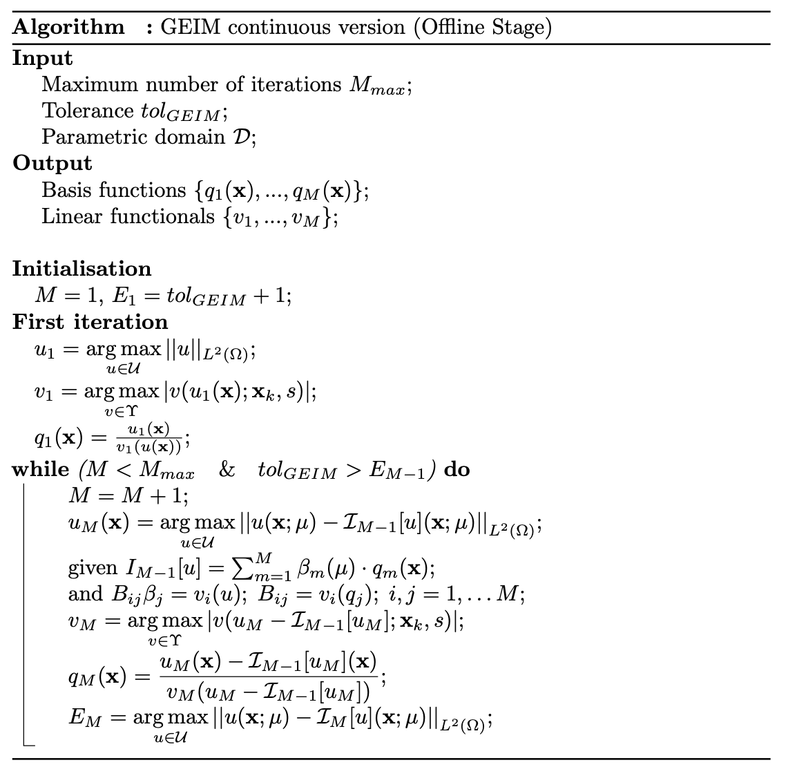
More information about the method can be found in Maday et al. (2014) and Introini et al. (2023).

Generation of the magic functions/sensors

The GEIM is used to generated through a greedy process a set of basis functions and basis sensors for the data assimilation process.

Sensors are mathematically modelled as linear continuous functionals \(v_m(\cdot)\), defined as \begin{equation*} v_m(u(\mathbf{x});\,\mathbf{x}_m,\,s)=\int_\Omega u(\mathbf{x})\cdot \mathcal{K}\left(\|\mathbf{x}-\mathbf{x}_m\|_2, s\right)\,d\Omega \end{equation*} given \(\mathbf{x}_m\) the centre of mass of the functional and \(s\) its point spread. The current version adopts Gaussian kernels \begin{equation*} \mathcal{K}\left(\|\mathbf{x}-\mathbf{x}_m\|_2, s\right) = \frac{e^{\frac{-\|\mathbf{x}-\mathbf{x}_m\|_2^2}{2s^2}}}{\displaystyle\int_\Omega e^{\frac{-\|\mathbf{x}-\mathbf{x}_m\|_2^2}{2s^2}}\,d\Omega} \end{equation*} such that \(\|\mathcal{K}\left(\|\mathbf{x}-\mathbf{x}_m\|_2, s\right)\|_{L^1(\Omega)}=1\), this models the measurement process of scalar fields.

A dictionary will be created for each GEIM with the keys consistent with the var_names variable. Moreover, the GEIM coefficients will be stored in a dictionary with the same keys: these will be needed in the online phase when the measures are polluted by random noise, within the Tikhonov Regularised version of the GEIM algorithm (TR-GEIM), Introini et al. (2023).

geim_data = dict()
train_GEIMcoeff = dict()

As for the POD in the previous notebook, the maximum number of sensors will be 20. The sensors are characterised by an hyperparameter, the spread \(s\), which depends on the specific sensor: two different values will be considered to investigate what is the effect on the reduction process.

Mmax = 20

s = [2, 5]
train_abs_err = np.zeros((Mmax, len(var_names), len(s)))
train_rel_err = np.zeros((Mmax, len(var_names), len(s)))

Here in this cell the GEIM class is defined, which will be used to generate the magic functions and sensors. The essential input of the GEIM class is the domain from which candidate positions are selected, the functional space, the name of the variable to analyse and the point spread \(s\) of the sensors.

from pyforce.offline.geim import GEIM

# This parameter serves as input to select only some cells in the mesh
# It is used to reduce the computational cost of the offline phase
sam_every = 4

for ii in range(len(var_names)):
    geim_data[var_names[ii]] = list()
    train_GEIMcoeff[var_names[ii]] = list()

    for jj in range(len(s)):

        # Define the GEIM object
        geim_data[var_names[ii]].append(GEIM(domain, V, var_names[ii], s=s[jj]))

The offline method is used to generate the magic functions and sensors: it requires as input the train snapshot, the maximum number of sensors to generate. sampleEvery and verbose are optional parameters.

for ii in range(len(var_names)):
    for jj in range(len(s)):

        print('--> '+var_names[ii]+' - s = {:.2e}'.format(s[jj]))

        # Perform the offline phase of GEIM
        tmp = geim_data[var_names[ii]][jj].offline(train_snaps[ii], Mmax,
                                                   sampleEvery = sam_every, verbose = True)

        # Store output
        train_abs_err[:, ii, jj] = tmp[0].flatten()
        train_rel_err[:, ii, jj] = tmp[1].flatten()
        train_GEIMcoeff[var_names[ii]].append(tmp[2])
        print(' ')
    print(' ')

--> phi_1 - s = 2.00e+00
Generating sensors (sampled every 4 cells): 1718.000 / 1718.00 - 0.003 s/it
  Iteration 020 | Abs Err: 2.41e-04 | Rel Err: 4.68e-06
--> phi_1 - s = 5.00e+00
Generating sensors (sampled every 4 cells): 1718.000 / 1718.00 - 0.004 s/it
  Iteration 020 | Abs Err: 1.54e-04 | Rel Err: 2.97e-06

--> phi_2 - s = 2.00e+00
Generating sensors (sampled every 4 cells): 1718.000 / 1718.00 - 0.005 s/it
  Iteration 020 | Abs Err: 3.28e-04 | Rel Err: 1.04e-05
--> phi_2 - s = 5.00e+00
Generating sensors (sampled every 4 cells): 1718.000 / 1718.00 - 0.003 s/it
  Iteration 020 | Abs Err: 3.53e-04 | Rel Err: 1.11e-05

Let us store the magic functions and the magic sensors

if not os.path.exists(path+'BasisSensors/'):
    os.makedirs(path+'BasisSensors/')
if not os.path.exists(path+'BasisFunctions/'):
    os.makedirs(path+'BasisFunctions/')
if not os.path.exists(path+'coeffs/'):
    os.makedirs(path+'coeffs/')

for ii in range(len(var_names)):
    for jj in range(len(s)):
        np.savetxt(path+'coeffs/GEIM_'+ var_names[ii] + '_s_{:.2e}'.format(s[jj])+'.txt', train_GEIMcoeff[var_names[ii]][jj],  delimiter=',')
        store(domain, geim_data[var_names[ii]][jj].magic_fun,  'GEIM_' +var_names[ii]+'_s_{:.2e}'.format(s[jj]), path+'BasisFunctions/basisGEIM_' + var_names[ii]+'_s_{:.2e}'.format(s[jj]))
        store(domain, geim_data[var_names[ii]][jj].magic_sens, 'GEIM_' +var_names[ii]+'_s_{:.2e}'.format(s[jj]), path+'BasisSensors/sensorsGEIM_' + var_names[ii]+'_s_{:.2e}'.format(s[jj]))

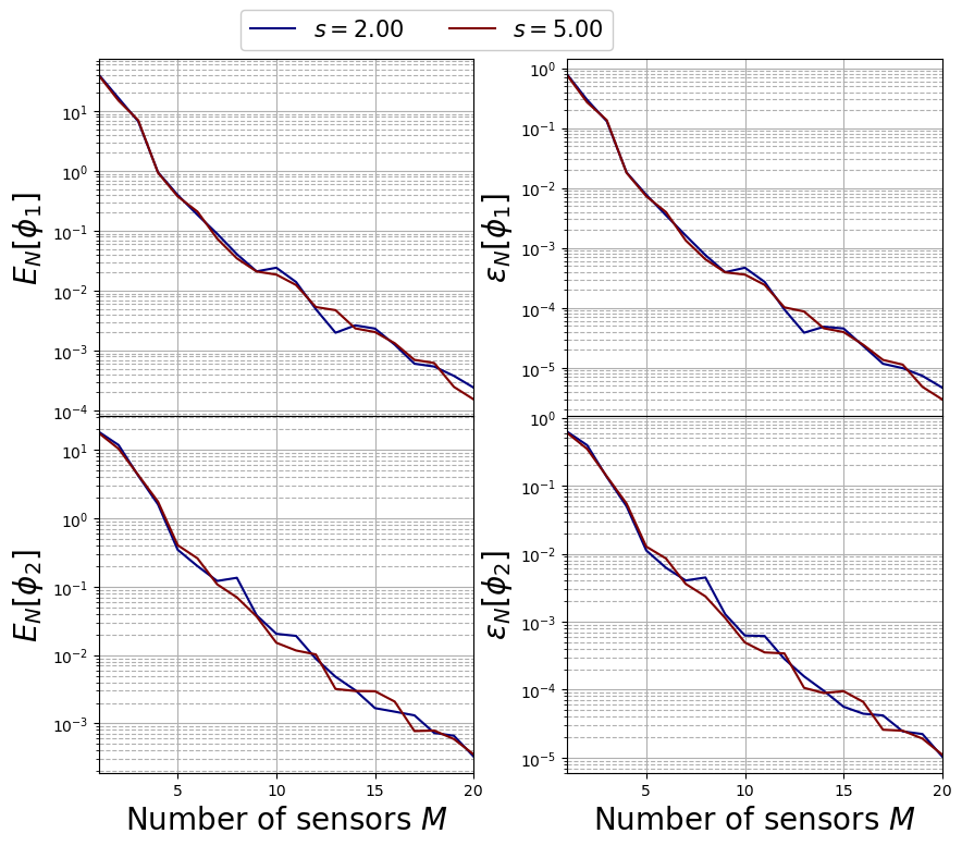
Comparison of the training errors

The max absolute and relative reconstruction error is compared for the different algorithms, given the following definitions \begin{equation*} \begin{split} E_M[u] &= \max\limits_{\boldsymbol{\mu}\in\Xi^{train}} \left\| u(\cdot;\,\boldsymbol{\mu}) - \mathcal{P}_M[u](\cdot;\,\boldsymbol{\mu})\right\|_{L^2(\Omega)}\\ \varepsilon_M[u] &= \max\limits_{\boldsymbol{\mu}\in\Xi^{train}} \frac{\left\| u(\cdot;\,\boldsymbol{\mu}) - \mathcal{P}_M[u](\cdot;\,\boldsymbol{\mu})\right\|_{L^2(\Omega)}}{\left\| u(\cdot;\,\boldsymbol{\mu}) \right\|_{L^2(\Omega)}} \end{split} \end{equation*} given \(\mathcal{P}_M\) the reconstruction operator with \(M\) magic functions (takes the reduced coefficients generated by GEIM and performs the linear combination of the magic functions).

TrainingErrFig, axs = plt.subplots(nrows = len(var_names), ncols = 2, sharex = True, figsize = (10,8) )

M = np.arange(1,Mmax+1,1)

for ii in range(len(var_names)):

    colors = cm.jet(np.linspace(0,1,len(s)))
    for jj in range(len(s)):
        axs[ii, 0].semilogy(M, train_abs_err[:Mmax, ii, jj], c=colors[jj], label = r'$s={:.2f}'.format(s[jj])+'$')
        axs[ii, 1].semilogy(M, train_rel_err[:Mmax, ii, jj], c=colors[jj], label = r'$s={:.2f}'.format(s[jj])+'$')

    axs[ii, 0].set_xticks(np.arange(0,Mmax+1,5))
    axs[ii, 0].set_xlim(1,Mmax)
    axs[ii, 0].set_ylabel(r"$E_N["+tex_var_names[ii]+"]$",fontsize=20)
    axs[ii, 1].set_ylabel(r"$\varepsilon_N["+tex_var_names[ii]+"]$",fontsize=20)

axs[1, 0].set_xlabel(r"Number of sensors $M$",fontsize=20)
axs[1, 1].set_xlabel(r"Number of sensors $M$",fontsize=20)

for ax in axs.flatten():
    ax.grid(which='major',linestyle='-')
    ax.grid(which='minor',linestyle='--')

Line, Label = axs[0,0].get_legend_handles_labels()

TrainingErrFig.legend(Line, Label, fontsize=15, loc=(0.25,0.94), ncols = len(s), framealpha = 1)
TrainingErrFig.subplots_adjust(hspace = 0, wspace=0.25, top = 0.93)

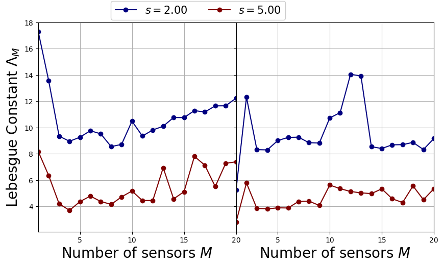
Calculation of the Lebesgue Constant

The Lebesgue Constant \(\Lambda_M\) is important for the GEIM algorithm, since it appears in the a-priori error estimation for the reduction technique. The procedure on how this is computed was introduced in Maday et al., (2015).

The Lebesgue constant can be computed using the function computeLebesgue: it requires the magic functions and the magic sensors as input.

from pyforce.offline.geim import computeLebesgue

Lebesgue_const = np.zeros((Mmax, len(var_names), len(s)))

bar = LoopProgress('Computing Lebesgue', final = len(var_names) * len(s))

for field_i in range(len(var_names)):
    for jj in range(len(s)):
        Lebesgue_const[:, field_i, jj] = computeLebesgue(geim_data[var_names[field_i]][jj].magic_fun,
                                                        geim_data[var_names[field_i]][jj].magic_sens)

        bar.update(1, percentage=False)

Computing Lebesgue: 4.000 / 4.00 - 4.632 s/it

Let us plot it to see the effect of the point spread

LebesgueFig, axs = plt.subplots(nrows = 1, ncols = 2, sharex = True, sharey = True, figsize = (10,5) )

for field_i in range(len(var_names)):
    colors = cm.jet(np.linspace(0,1,len(s)))
    for jj in range(len(s)):
        axs[field_i].plot(M, Lebesgue_const[:, field_i, jj], '-o', c=colors[jj], label = r'$s={:.2f}'.format(s[jj])+'$')

    axs[field_i].set_xlabel(r"Number of sensors $M$",fontsize=20)
    axs[field_i].grid(which='major',linestyle='-')
    axs[field_i].grid(which='minor',linestyle='--')

    axs[field_i].set_xticks(np.arange(0, Mmax+1,5))
    axs[field_i].set_xlim(1, Mmax)

axs[0].set_ylabel(r"Lebesgue Constant $\Lambda_M$",fontsize=20)
for ax in axs.flatten():
    ax.grid(which='major',linestyle='-')
    ax.grid(which='minor',linestyle='--')

Line, Label = axs[0].get_legend_handles_labels()

LebesgueFig.legend(Line, Label, fontsize=15, loc=(0.25,0.925), ncols = len(s), framealpha = 1)
LebesgueFig.subplots_adjust(hspace = 0, wspace=0, top = 0.93)

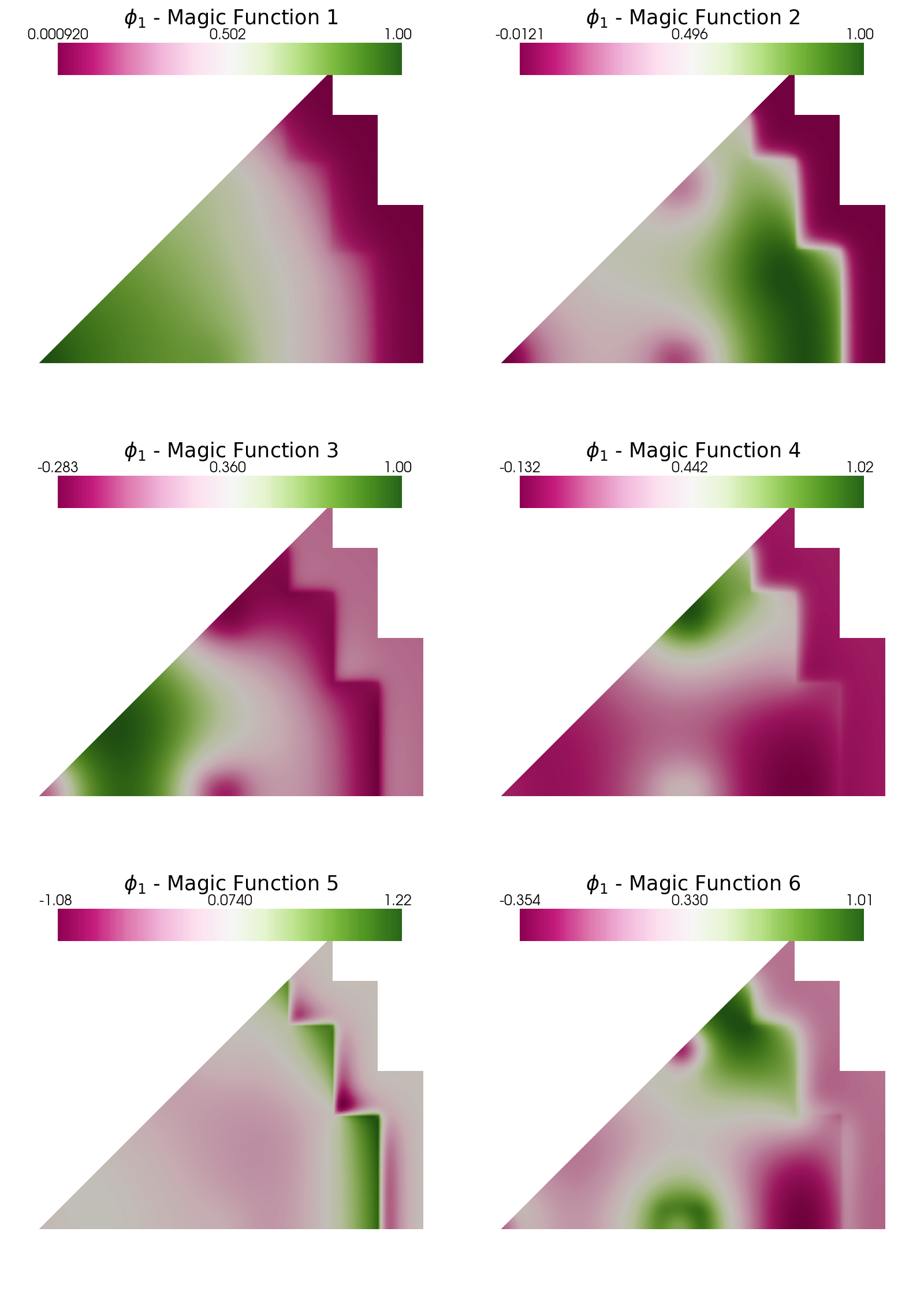
Post Process

In this last section, pyvista is used to make some contour plots of the magic functions and sensors for the fast and thermal flux.

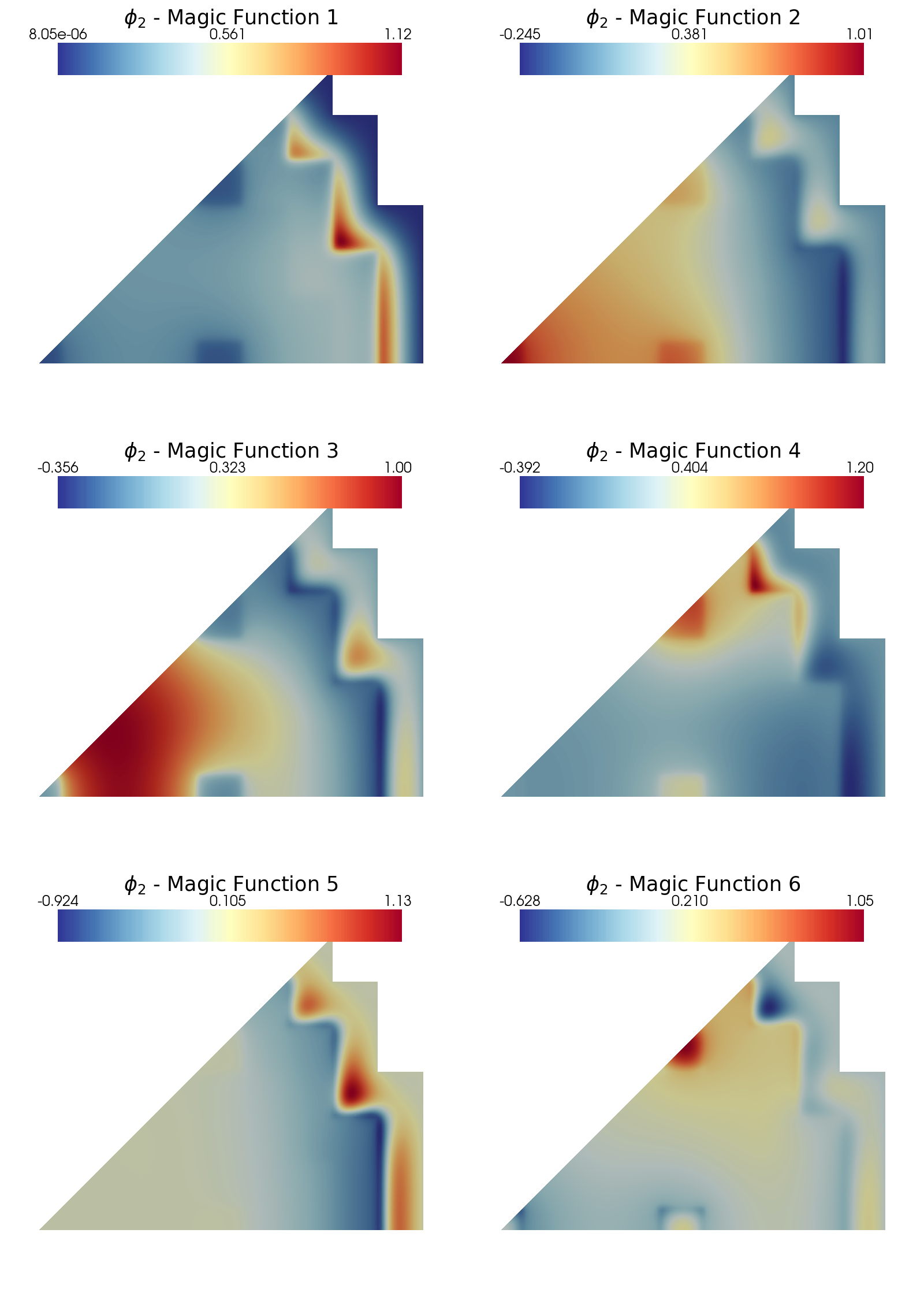
Let us plot the first 6 magic functions of each variable, for \(s=2\): in particular, contour plots of the fast and thermal flux are shown.

from contour_plotting import plot_modes

plot_modes(geim_data[var_names[0]][0].magic_fun, tex_var_names[0],
           shape = [3,2], colormap=cm.PiYG, title = 'Magic Function')
plot_modes(geim_data[var_names[1]][0].magic_fun, tex_var_names[1],
           shape = [3,2], colormap=cm.RdYlBu_r, title = 'Magic Function')

In the end, let us plot the sensors positions for the fast and thermal flux, for each value of \(s\).

from contour_plotting import plot_geim_sensors

plot_geim_sensors(geim_data[var_names[0]], 15, [r'$s={:.2f}$'.format(ss) for ss in s], 0, cmap=cm.hot)
plot_geim_sensors(geim_data[var_names[1]], 15, [r'$s={:.2f}$'.format(ss) for ss in s], 1, cmap=cm.cool)

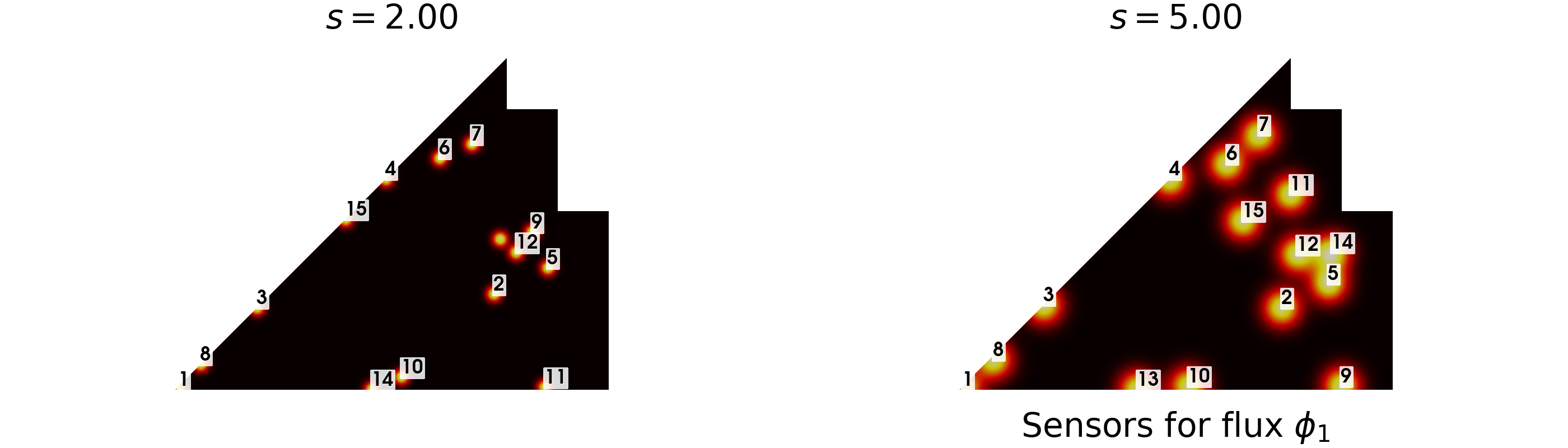
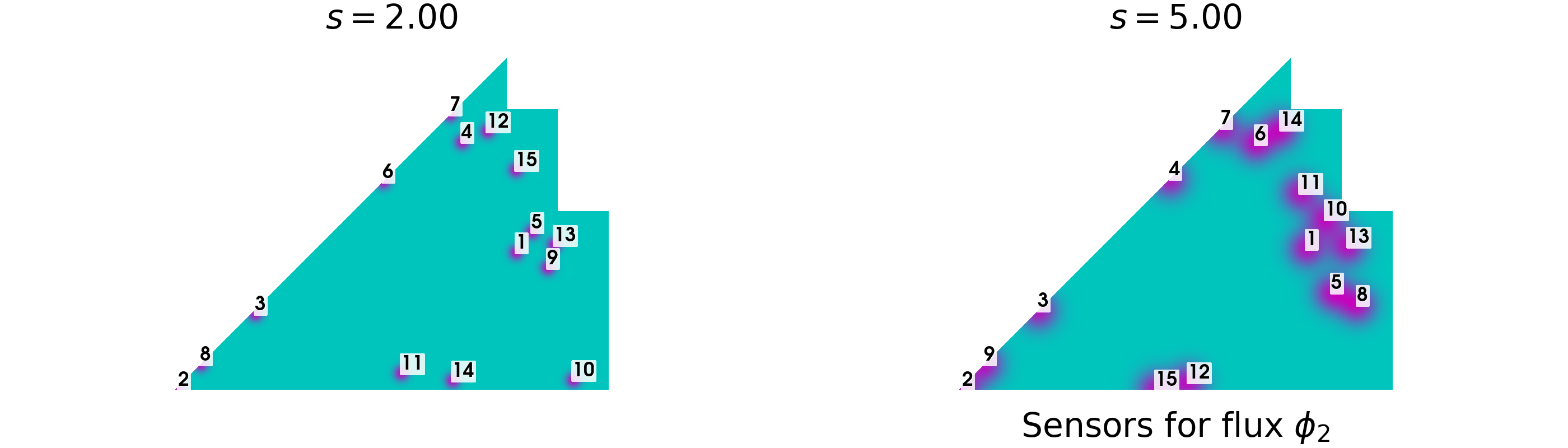
The first 3 positions are identical for the two values of \(s\), then some differences are observed. In the coming notebooks, only the case with \(s=2\) will be considered since better represents the reality of a flux sensors.