Importing Snapshots from OpenFOAM
Aim of this notebook: learn how to import transient snapshots from OpenFOAM (version 2012 from com-version) using pyvista package.
The snapshots are related to the laminar Flow Over Cylinder in fluid dynamics, governed by the Navier-Stokes equations. In particular, the snapshots have been generated using the tutorial case reported here. Furthermore, some features of the pyvista package are shown, including plotting and data manipulation.
The data are available on Zenodo, change the folder name to OF_case or change the path in the code below.
The class ReadFromOF is used to read the OpenFOAM snapshots, create a mesh for dolfinx and plot the results using pyvista.
[1]:
from pyforce.tools.write_read import ReadFromOF

of = ReadFromOF('OF_case/')
/Users/sriva/miniconda3/envs/ml/lib/python3.10/site-packages/ufl/__init__.py:244: UserWarning: pkg_resources is deprecated as an API. See https://setuptools.pypa.io/en/latest/pkg_resources.html. The pkg_resources package is slated for removal as early as 2025-11-30. Refrain from using this package or pin to Setuptools<81.
  import pkg_resources
The case contains an UnstructuredGrid element containing the fields U, p. The default time step is 0, but you can change it to any other time step available in the case.
[2]:
of.reader.read()
[2]:
| Information | Blocks | |||||||||||||||||||
|---|---|---|---|---|---|---|---|---|---|---|---|---|---|---|---|---|---|---|---|---|
|
|
The time instants saved can be printed
[3]:
import numpy as np

times = np.array(of.reader.time_values)
print('Time values:', times)
Time values: [  0.   2.   4.   6.   8.  10.  12.  14.  16.  18.  20.  22.  24.  26.
  28.  30.  32.  34.  36.  38.  40.  42.  44.  46.  48.  50.  52.  54.
  56.  58.  60.  62.  64.  66.  68.  70.  72.  74.  76.  78.  80.  82.
  84.  86.  88.  90.  92.  94.  96.  98. 100. 102. 104. 106. 108. 110.
 112. 114. 116. 118. 120. 122. 124. 126. 128. 130. 132. 134. 136. 138.
 140. 142. 144. 146. 148. 150. 152. 154. 156. 158. 160. 162. 164. 166.
 168. 170. 172. 174. 176. 178. 180. 182. 184. 186. 188. 190. 192. 194.
 196. 198. 200. 202. 204. 206. 208. 210. 212. 214. 216. 218. 220. 222.
 224. 226. 228. 230. 232. 234. 236. 238. 240. 242. 244. 246. 248. 250.
 252. 254. 256. 258. 260. 262. 264. 266. 268. 270. 272. 274. 276. 278.
 280. 282. 284. 286. 288. 290. 292. 294. 296. 298. 300. 302. 304. 306.
 308. 310. 312. 314. 316. 318. 320. 322. 324. 326. 328. 330. 332. 334.
 336. 338. 340. 342. 344. 346. 348. 350. 352. 354. 356. 358. 360. 362.
 364. 366. 368. 370. 372. 374. 376. 378. 380. 382. 384. 386. 388. 390.
 392. 394. 396. 398. 400. 402. 404. 406. 408. 410. 412. 414. 416. 418.
 420. 422. 424. 426. 428. 430. 432. 434. 436. 438. 440. 442. 444. 446.
 448. 450. 452. 454. 456. 458. 460. 462. 464. 466. 468. 470. 472. 474.
 476. 478. 480. 482. 484. 486. 488. 490. 492. 494. 496. 498. 500.]
In internalMesh, the fields are saved as point data or cell data, which can be used for plotting.
[4]:
import pyvista as pv
from IPython.display import clear_output as clc

dict_cb = dict( width = 0.65, height = 0.15,
                    n_labels=4,
                    color = 'k',
                    position_x=0.175, position_y=0.0785,
                    shadow=False)

tt = len(of.reader.time_values)-1

of.reader.set_active_time_value(of.reader.time_values[tt])
mesh = of.reader.read()['internalMesh']

pl = pv.Plotter(shape=(1, 2), border=False, off_screen=True, window_size=(1200, 400))

pl.subplot(0,0)
pl.add_mesh(mesh.slice(normal='z'), scalars='U', cmap='RdYlBu_r', scalar_bar_args=dict_cb)

pl.subplot(0,1)
pl.add_mesh(mesh.slice(normal='z'), scalars='p', cmap='viridis', scalar_bar_args=dict_cb)

for i in range(2):
    pl.subplot(0, i)
    pl.view_xy()
    pl.camera.zoom(2)

pl.add_text(f'Time = {of.reader.time_values[tt]} s', position='upper_edge', font_size=20, color='k')
pl.show(jupyter_backend='static')
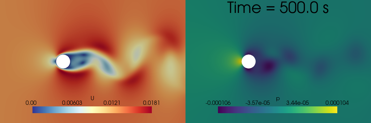
Let us import the velocity and pressure fields from the OpenFOAM case.
[5]:
var_names = ['U', 'p']
vector = [True, False]

of_snaps = dict()
for field_i, field in enumerate(var_names):
    of_snaps[field] = np.asarray(of.import_field(field, vector=vector[field_i])[0])
Importing U using pyvista
Importing p using pyvista
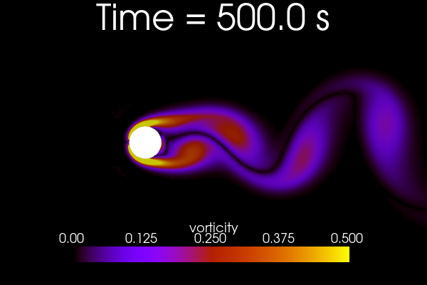
Let us add also the vorticity field, defined as the curl of the velocity field, \(\boldsymbol{\omega} = \nabla \times \mathbf{u}\).
[6]:
from pyforce.tools.backends import LoopProgress

var_names.append('vorticity')
vector.append(True)

of_snaps['vorticity'] = np.zeros_like(of_snaps['U'])

bar = LoopProgress(msg='Computing vorticity', final =of_snaps['U'].shape[0])
for tt in range(of_snaps['U'].shape[0]):

    of.reader.set_active_time_value(of.reader.time_values[tt])
    mesh = of.reader.read()['internalMesh']
    of_snaps['vorticity'][tt] = mesh.compute_derivative(scalars='U', vorticity=True)['vorticity']

    bar.update(1)
Computing vorticity: 250.000 / 250.00 - 0.215 s/it
Let us make a plot of the vorticity field using pyvista.
[18]:
dict_cb = dict( width = 0.65, height = 0.15,
                    n_labels=5,
                    color = 'white',
                    position_x=0.175, position_y=0.0785,
                    shadow=False)

tt = len(of_snaps['vorticity']) - 1

mesh = of.reader.read()['internalMesh']

mesh['vorticity'] = of_snaps['vorticity'][tt]

pl = pv.Plotter(window_size=(600, 400))
pl.add_mesh(mesh.slice(normal='z'), scalars='vorticity', cmap='gnuplot', scalar_bar_args=dict_cb, clim=(0,0.5))

pl.view_xy()
pl.camera.zoom(2)

pl.add_text(f'Time = {of.reader.time_values[tt+1]} s', position='upper_edge', font_size=20, color='white')

pl.show(jupyter_backend='static')
Let us save the snapshots in a npz file for later use.
[23]:
path_snaps = 'Snapshots/'
import os
os.makedirs(path_snaps, exist_ok=True)

np.savez_compressed(path_snaps+'of_dataset.npz', snaps=of_snaps, time_values=times[1:], is_vector=vector, var_names=var_names)
Let us store also the mesh in a vtk file for later use.
[27]:
mesh = of.reader.read()['internalMesh']
mesh.clear_data()
mesh.save(path_snaps+'of_mesh.vtk')